This page describes the JOREK setup for free-boundary mode that are common for both STARWALL and CARIDDI. In this page you will find
What do I need to run JOREK in free-boundary mode?
- A wall-vacuum response file within the JOREK running directory. For STARWAL this file's name is starwall-response.dat, which is computed by STARWALL.
- Set specific input parameters in the JOREK input file.
See this tutorial to get started.
Getting the response file
- Run JOREK with
freeboundary=.t.in the input file. JOREK will stop and the boundary.txt file with the geometry of the coupling surface will appear in the folder. - Copy boundary.txt to the STARWALl or CARIDDI run folder.
- Run STARWALL or Run CARIDDI
- Copy the response.dat file produced by STARWALL or CARIDDI in the JOREK running directory
JOREK input file free-boundary parameters
Main parameters
| Parameter | Description | |-----------|-------------| | freeboundary | Run with free-boundary activated | | freeboundary_equil | Run a free boundary equilibrium instead of a fixed boundary equilibrium, see free-boundary equilibrium. | | wall_resistivity_fact | Scale wall and coil resistivities by this factor (default=1.0). The nominal wall and coil resistivity is setup in the input files of STARWALL and CARIDDI |
Coil current parameters
Sometimes coil currents are needed to run, for example to compute a free-boundary equilibrium or to do RMP studies. For each coil, the time trace of the current evolution (in Amperes/turn) can be prescribed in the JOREK namelist input file. This is done separately for:
rmp_coils(*)pf_coils(*)
Note: The
voltage_coilsare not yet completely implemented, and fordiag_coilsprescribing a current is usually not useful.
Sign convention: is such that a positive current in the input file follows the positive phi direction as in the JOREK coordinate system.
IMPORTANT: If you want the coils to have the exact currents you prescribe, you must set the coil resistance with a very high value (around
1.d0will be ok). The coil currents will decay to the prescribed currents in the resistive time of the coils. See the Run STARWALL or Run CARIDDI for more information.
There are several ways for prescribing the current time trace. The following examples illustrate different approaches:
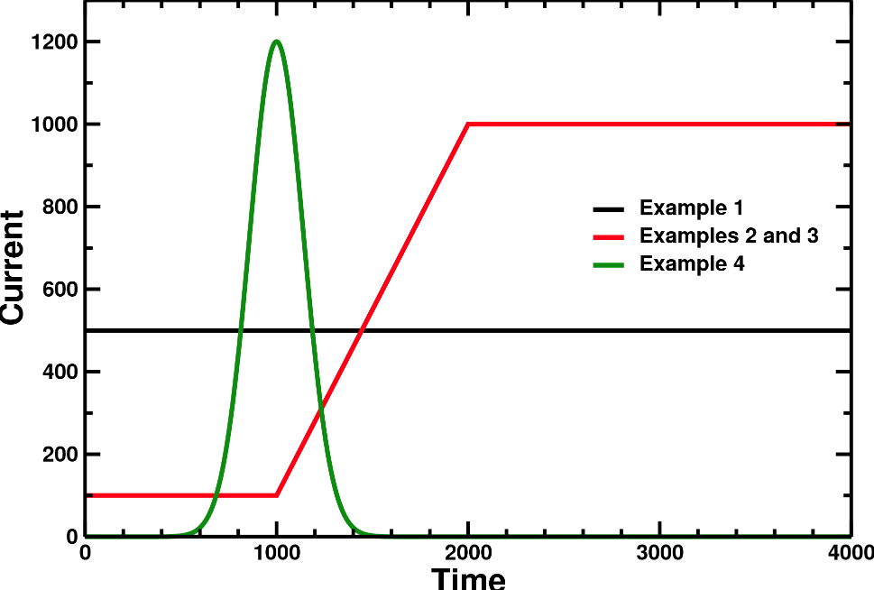
1) Constant in time
rmp_coils(1)%current = 500.
2) Constant in time plus a perturbation
rmp_coils(1)%current          = 100.
rmp_coils(1)%pert             = 1000.
rmp_coils(1)%pert_start_time  = 1000.
rmp_coils(1)%pert_growth_time = 1000.
The current is ramped up linearly from current to current+pert from time pert_start_time to pert_start_time+pert_growth_time and then remains constant.
3) Prescribed by an ASCII file
rmp_coils(1)%curr_file = 'file_name'
The file needs to contain time points in the first column and current values in the second column. Example:
0.    100.
1000. 100.
2000. 1000.
1.e5  1000.
4) Analytical expression
rmp_coils(1)%curr_expr = '1200*exp(-(t-1000.)**2/(200.)**2)'
rmp_coils(1)%max_time  = 10000.
rmp_coils(1)%len       = 2000
An analytical expression can be provided and is evaluated at the beginning of the simulation by calling Python. It is important to specify:
max_time: covers the complete simulation timelen: number of points the expression is evaluated on
In the example, the expression is evaluated on 2000 points between t=0 and t=10000. Set max_time and len carefully!
Additional modifiers
Scale the time, shift the time, and scale the amplitude using the following parameters:
rmp_coils(1)%time_scale  = 2.d0   ! slow down current evolution by factor two
rmp_coils(1)%time_shift  = 100.   ! shift the current evolution to take place dt=100 later
rmp_coils(1)%curr_scale  = 2.d0   ! increase currents by factor two
For time, the scaling factor is applied first, then the shift.
Visualizing coil currents with plot_live_data.sh:
The input of the coils in the JOREK input files is done in amperes/turn (see above). However, the output in plot_live_data.sh is normalized by $I_{SI} = I/\mu_0$. You can plot the time trace with plot_live_data.sh with -q pf_coil, -q rmp, -q diag for the PF coils, RMP, coils and diagnostic coils respectively.
Free-boundary equilibrium parameters and advices
To run a free-boundary equilibrium, include the mode n=0 in the response file. You also need a separate to specify the corresponding equilibrium coils in either STARWALL or CARIDDI.
With the correct response file, set the coil currents and free-boundary equilibrium parameters in the JOREK input file:
freeboundary = .t.
freeboundary_equil = .t.

pf_coils(1)%current     =  2.6d+4     ! Amperes/turn
pf_coils(2)%current     = -2.6d+4
pf_coils(3)%current     =  1.0d+4
pf_coils(4)%current     =  1.0d+4

amix_freeb = 0.d0        ! To speed up convergence

use_mumps_eq = .t.       ! Optional, but works much faster than Pastix 5

cte_current_FB_fact = 1. ! Multiplies T and FF' profiles with this factor at start of freebnd iterations
Run the equilibrium. If coil geometry and currents are correct, it should converge. First, verify that the fixed boundary equilibrium converges to the right solution before running on free-boundary. If you experience convergence problems in free-boundary mode:
- Try increasing
amix_freebto values between 0.5 and 0.9 (helps when the fixed boundary equilibrium differs from the free-boundary solution) - Use
cte_current_FB_factto scale the current density profile to obtain the desired final total plasma current
OLD: Controlling total current and vertical position during Grad-Shafranov (Picard) iterations
To use the old Picard iterations with feedback on vertical position and total current, set in the JOREK input file:
newton_GS_freebnd = .f.
This feature remains useful if you want to impose a given plasma current and vertical position.
Free-boundary equilibrium computations require active feedback on the plasma total current ($I_p$) and vertical position ($Z_{axis}$ if vertically unstable) during Picard iterations. Tune these feedback parameters for convergence:
| Parameter | Description |
|---|---|
current_ref | Target total plasma current (wished final current in Amperes) |
n_feedback_current | Apply $I_p$ feedback each "n" Picard iterations |
FB_Ip_position | Strength of $I_p$ correction per iteration, proportional to $(I_p - I_{p,ref})$ (experimental values: 0.1–2.0) |
FB_Ip_integral | Integral feedback parameter for $I_p$ correction, accounts for feedback history (experimental values: ~0.01) |
Z_axis_ref | Target $Z$ position of the magnetic axis (in meters) |
n_feedback_vertical | Apply $Z_{axis}$ feedback each "n" Picard iterations |
FB_Zaxis_position | Strength of $Z_{axis}$ correction per iteration, proportional to $(Z_{axis} - Z_{axis,ref})$ (experimental values: 1.0–20.0) |
FB_Zaxis_integral | Integral feedback parameter for $Z_{axis}$ correction (experimental values: ~0.01) |
FB_Zaxis_derivative | Derivative feedback parameter, proportional to $Z_{axis}-Z_{axis,old}$, where $Z_{axis,old}$ is the previous iteration position |
start_VFB | Iteration number at which to begin $Z_{axis}$ feedback |
Indicate which coils are used for vertical feedback:
vert_FB_amp(3) = -1.d0
vert_FB_amp(4) =  2.5d0
The coil number 4 will increase its current if plasma moves upwards (positive sign). Use minus sign for upper coils and plus for lower coils. The value 2.5 indicates relative feedback strength—coil 4 current changes 2.5 times faster than coil 3. Set to 0.0 to disable feedback for a coil.
Other useful free-boundary equilibrium parameters
| Parameter | Description |
|---|---|
n_iter_freeb | Maximum number of iterations for the free-boundary equilibrium |
amix_freeb | Mixing factor for free-boundary equilibrium; range (0.5–0.95) depending on case complexity |
equil_accuracy_freeb | Convergence tolerance (1.d-6 is reasonable) |
freeb_equil_iterate_area | Limiter plasmas only. Defines plasma boundary as the flux contour enclosing the final plasma area from fixed-boundary equilibrium. With $I_p$ feedback, ensures plasma resembles fixed-boundary solution (same area, same $I_p$) |
psi_offset_freeb | Shift psi by a global constant to smooth transition between fixed-boundary and free-boundary equilibrium |