Generating Poincaré Plots with Particle Tracker
What's different to jorek2_poincare
- Option to generate Poincaré plots with particles and not just field lines.
- Output is separated for each marker and includes connection length.
- Output is stored in HDF5 format.
1. Compiling and running the code
- It is recommended to use MUMPS for the particle tracer (set
USE_MUMPS=1inMakefile.inc). - (For plotting you will need numpy, h5py, and matplotlib)
- Compile the Poincaré program with:
make poincare - Include the binary in the same folder with JOREK inputs and restart files.
-
The simulation options are given in
pncrfile which you should also include in the same folder and contains the following:# n_tracers - number of field line/particle tracers 100 # n_turns - how many times a marker must cross the outer mid-plane before terminating its simulation 200 # tstep in [s] for particles and [m] for field lines (1e-3 - 1e-2 is good for field lines, for particles it depends but 1e-8 - 1e-10 is ok for electrons) 1.0e-10 # mass [AMU] (if you use 0.0 here then field lines are traced) 0.00055 # charge [e] -1 # pitch (vpar/vtot) 0.99 # energy [eV] 1.0e3 - You can change the values in
pncrfile but don't alter the structure. - The Poincaré data is collected for a single time-slice that corresponds to
jorek_restart.h5. - To run the code, use
mpirun -n 1 ./poincare < input_namelist
Further information and possible issues
- Issues can arise if time-step is too large (e.g. field lines diverge or have “width” in the plot or the simulation might not complete). Reducing time-step means simulations take longer time, but you can alleviate this by reducing
n_tracersandn_turns. Running with default settings should take just few minutes. - Tracing particles by default includes electric field, which can cause acceleration. To disable the electric field, add
E=0at the end of the subroutinecalc_EBNormBGradBCurlbDbdtinparticles/mod_fields.f90. - When tracing particles, relativistic guiding center pusher is used. This could be an issue when the guiding center approximation is not valid e.g. in spherical tokamaks.
- Markers are initialized at the outer mid-plane at even intervals radially, and the initial toroidal angle is randomly sampled from uniform distribution.
- Field lines are traced in one direction along the B-field vector. For particles this is determined by pitch.
2. Compiling and running the code
- The program outputs
poincare.h5fiel that contains the following fields
r       : R-coordinate
z       : z-coordinate
phi     : Toroidal angle [rad]
psi     : Normalized psi
iprt    : Marker ID this data point correspond to (1,...,Nmrk)
pncrid  : Poincare plane this data point correspond to (default is phi-tor plane = 1 and Rz-plane = 2 )
mil     : Distance the marker has travelled up to this point
mileage : The distance [m] that a marker travelled in total
- The data is stored in unstructured 1D arrays where each data point corresponds to a crossing of poloidal or toroidal plane. This makes it easy to modify the code so that the data is collected in several (poloidal or toroidal) planes simultaneously.
iprtandpncridcan be used to disect the data. For example, to get indices of all points for marker i at plane j, use:idx = np.logical_and.reduce([iprt == i, iplane == j])-
At the moment the data is collected at Rz-plane corresponding to phi = 0, and at the outer mid-plane. The results can be visualized with
util/plot_poincare.pyjust by running the script. Here's an example output: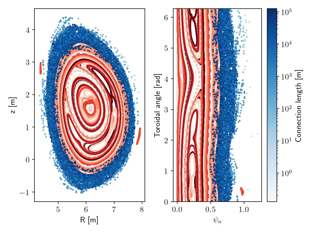
- The colors in red hue indicate confined markers (ones that were not lost during the simulation). Each marker is assigned a (red tinted) color from a pool of six colors, which makes it easier to separate adjacent lines.
- The colors in blue hue indicate connection length of the lost markers. The color shows the connection length at that position