Running the stellarator model with a divertor region
Unlike tokamak models, JOREK does not have a built-in equilibrium solver for stellarator but uses an ideal MHD equilibrium solver from GVEC, assuming nested flux surfaces. Historically, this meant that the simulation domain has been limited to the Last Closed Flux Surface (LCFS). To go beyond the LCFS, one typically either needs:
- Dommaschk potentials
- Vacuum field $\nabla \chi$ from coils
For further conceptual details, see the stellarator page. This page illustrates the minimal building blocks to get started with creating and running simulations with stellarator grids with divertors.
For the baseline stellarator import chain (GVEC to JOREK restart files), first see Run Stellarator Simulations.
Minimal context for this page:
- Start from
gvec2jorek.dat(or its modified variant). - Run model 180 to build a consistent restart state (
jorek000000.h5,jorek000001.h5). - Use
jorek000001.h5asjorek_restart.h5for model 183.
USE_EXT_FIELD controls where the vacuum field used by stellarator boundary diagnostics/BCs comes from:
USE_EXT_FIELD=0: use the chi-based pathway (no explicitB_vac_*arrays required ingvec2jorek.dat).USE_EXT_FIELD=1: use explicit vacuum-field arrays (B_vac_R,B_vac_Z,B_vac_phiand derivatives) ingvec2jorek.dat.
For W7-X divertor workflows where coil-field topology at the boundary is required, this page assumes USE_EXT_FIELD=1 and a gvec2jorek.dat that already contains B_vac_* blocks.
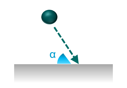
To realistically capture divertor physics, sheath boundary conditions (SBC) are necessary to capture the dynamics close to the first wall when open magnetic field intersect the boundary. The well-established main physics formulae, already implemented in the JOREK tokamak model and in other divertor physics codes, state that for flux surfaces intersecting boundaries with angle $\alpha$, we have (where $\alpha_0$ can bet set to e.g. 5 deg):
- The Bohm criterion:
-
Particle flux at sheath entrance: $\Gamma_n = n \cdot v_{\parallel}$
-
Heat flux (simplest case with single $T$): $q = \gamma \cdot k T_e \Gamma_n$
More physics details on SBC and their implementation can be found in P.C Stangeby (2000), CRC Press, and M. Hoelzl et al., Nucl. Fusion 61, 065001 (2021). The stellarator model 183 now contains a working stellarator SBC path, but unlike tokamaks we must handle strongly 3D, toroidally varying incidence angles $\alpha(\theta,\phi)$ and represent BC targets consistently in the toroidal Fourier basis.
Simplistic case: W7-A with artificial divertor
The first minimum viable stellarator divertor grid example features an artificial divertor indentation in the stellarator Wendelstein 7-A (sketch for illustrative purposes only):
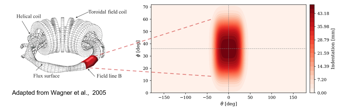
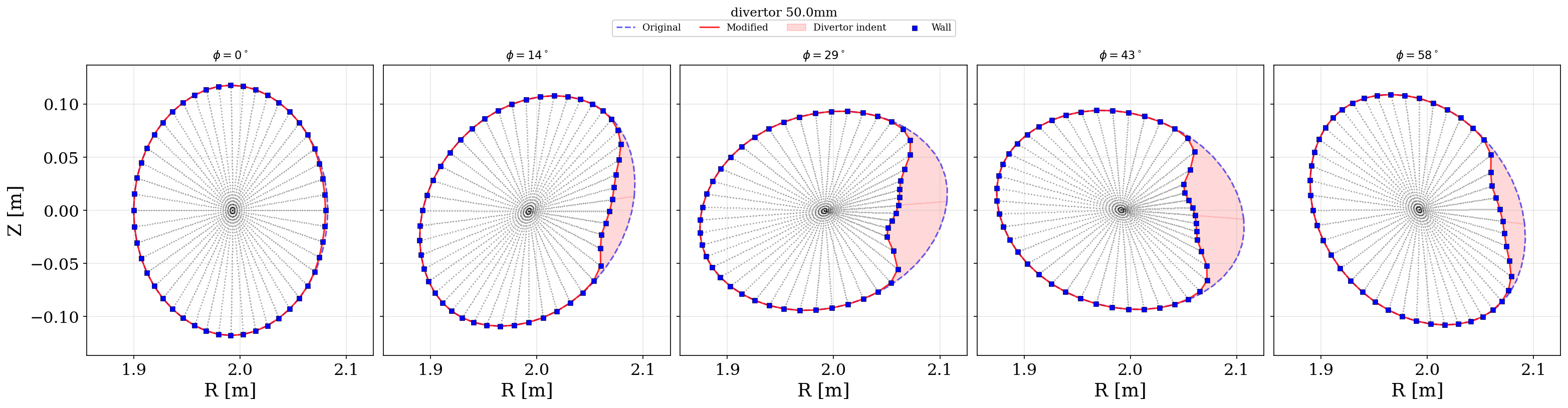
The indentation used is a smooth inward radial displacement of the boundary shell, with depth parameter $d$ (here $d=50$ mm, the more extreme test case). For this artificial W7-A test divertor, the indentation patch can be described analytically:
\[\Delta r(\theta,\phi) = d\,\frac{f_\theta(\theta)\,f_\phi(\phi)}{\sqrt{\cos^2\theta + \left(\sin\theta/\kappa\right)^2}}\]where $f_\theta$ and $f_\phi$ are tanh-window envelopes, based on smoothing functions:
def tanh_smooth(x, center, width, smooth_width):
    """Smooth envelope: 1 inside [center-width, center+width], 0 outside."""
    left = 0.5 * (1 + np.tanh((x - (center - width)) / smooth_width))
    right = 0.5 * (1 - np.tanh((x - (center + width)) / smooth_width))
    return left * right
and $\kappa$ is the ellipticity factor (in this example, $\kappa=1.5$). In practice, boundary nodes are moved inward by $\Delta r$ and interior shells are scaled proportionally from axis (0) to boundary (1). An example usage to plot this artificial indentation is found in W7-A example indentation map.
Bezier-Hermite handling in this W7-A step is intentionally simple: geometry is modified in real space and first/mixed derivatives (_s, _t, _st) are recomputed with scipy.interpolate.PchipInterpolator in radial and poloidal directions (including periodic closure in poloidal angle). This avoids stale handles after boundary displacement.
TO DO: when stellarator_setup.md done, link to this script.
The main ingredients can be found in the modify_w7a_gvec2jorek_to_divertor script. Inputs are the original gvec2jorek.dat geometry/Fourier fields and a geometric indentation prescription. Output is a modified gvec2jorek_divertor_<depth>mm.dat, then model180/model183 follow the standard chain from the stellarator set-up.
This step is a first direct geometry-indentation workflow for W7-A, to demonstrate grid modification principles before any bloating or harmonic mapping is needed.
W7-X divertor grids
Grid construction
Incorporating the vacuum field in the gvec2jorek.dat file
This step requires a) a functional gvec2jorek.dat equilibrium file and b) an mgrid file (containing the vacuum fields) from W7-X. If you do not have these files, reach out to the W7-X team.
TO DO: link to 1) mgrid_w7x.nc (high_res), 2) gvec2jorek.dat file and 3) W7-X divertor files in Kisslinger format if/when they become publicly available.
The vacuum field is added by sampling the W7-X mgrid coil field on the JOREK flux grid, transforming to toroidal Fourier modes, and appending B_vac_* blocks to gvec2jorek.dat. The reference script is w7x_mgrid2bvac. The script basically does the following:
- Read existing
gvec2jorek.datinto grid geometryR(s,theta,phi), Z(s,theta,phi) - Read
mgrid_w7x.ncintoB_vac(R,Z,phi)per coil group on cylindrical grid, sum coil contributions withEXTCURweights - interpolate mgrid
B(R,Z,phi) - Fourier transform in phi
- Write
B_vac_R/Z/phi(+_s,_t,_st) to gvec2jorek.dat
Remember that the mgrid file and EXTCUR values must correspond to the same magnetic configuration used to generate the target equilibrium (otherwise imported vacuum topology is inconsistent). Also, USE_EXT_FIELD=1 is necessary in the jorek model 180 / 183 compilation to include the vacuum field.
Harmonic mapping
Harmonic mapping - defined by two coordinate functions that are harmonic, constructed as the solution of two Laplace’s equations with Dirichlet boundary conditions - constructs smooth, nested extension shells in strongly non-axisymmetric geometry by solving the mapping problem per toroidal plane and then rebuilding a toroidally consistent Fourier representation. This method reduces geometric distortion and helps preserve positive Jacobians during extension, see details Robert Babin et al., Plasma Phys. Control. Fusion 67 (2025) 035005.
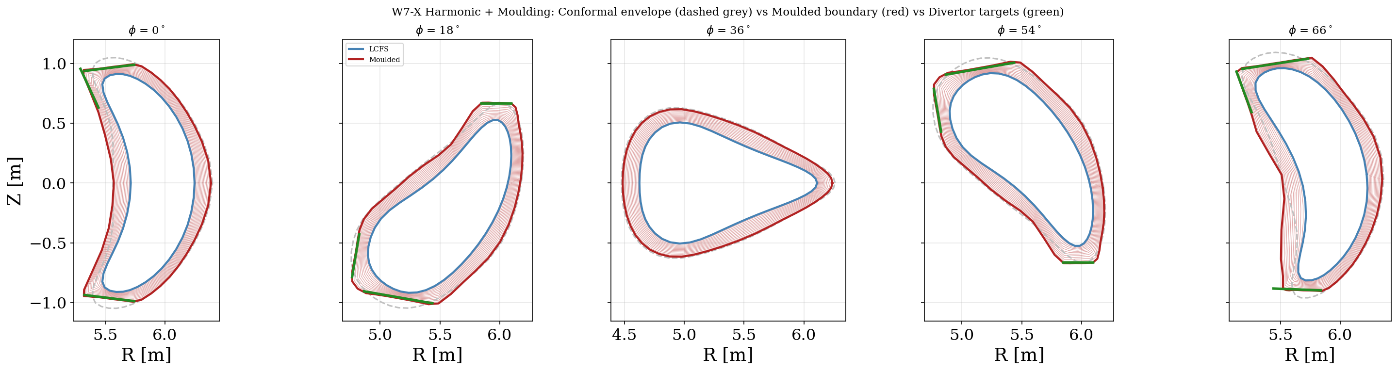
In w7x_extend_grid_harmonic.py, Step 1 is the harmonic mapping stage: for each toroidal plane, LCFS is mapped to an additive conformal envelope, then transformed back to Fourier modes over all planes.
Divertor moulding
In the same script, Step 2 is divertor moulding: a displacement/scale field is built from ray intersections with divertor target segments, then extension shells are rescaled toward those targets with smooth angular tapers (DIVERTOR_SMOOTH_DEG, PHI_TAPER_DEG) and safety bounds (SCALE_MIN, SCALE_MAX) to keep the mesh regular.
An example output plot of the constructed grid that extends all the way to the divertor surfaces can be seen below (also with the original LCFS marked, inside which the grid is virtually untouched):