Grad-Shafranov Tutorial
This tutorial describes how to reconstruct a Grad-Shafranov equilibrium in JOREK.
GS inputs
The Grad-Shafranov (GS) equation reads:
\[\Delta^{\ast}\psi = -\mu_0 R^{2}\displaystyle\frac{dp(\psi)}{d\psi} - F(\psi)\displaystyle\frac{dF(\psi)}{d\psi}\]where $p$ and $F$ are functions of $\psi$ of course.
There are three essential inputs required to solve the GS inside an ideal wall:
- pressure profile
- $FF'$ profile
- $\psi$-contour around the plasma
We will now go through each input and how to obtain it, based on experimental data. For this tutorial, we will use JET data, but in a generic manner, so that this can apply to any experimental input.
However, before starting, it should be noted that the simplest method to import data into a JOREK input file is to use the JOREK executable eqdsk2jorek, which takes an eqdsk equilibrium file as input. Some documentation about this tool can be found in the eqdsk2jorek page. It is helpful to be aware that very often a normalization factor of $ 2\pi $ is used for the poloidal magnetic flux $ \Psi = \psi/(2\pi)$ (this is the case when the COCOS number has two digits). When this is done, users should account for it both in the psi value on the boundary and in the ffprime profile (as F' is the derivative with respect to $\psi$ and not $\psi_\mathrm{norm}$).
The $\psi$-contour for the boundary conditions
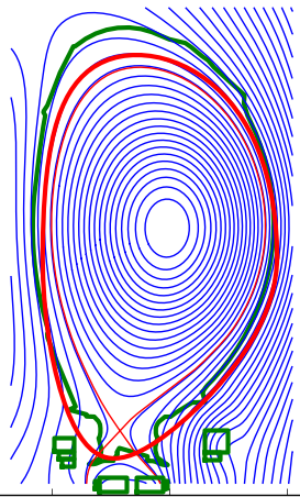
Given an eqdsk file, or any equilibrium input, a boundary is needed around the plasma, including the $\psi$-values for each point of the contour. The input to feed into the JOREK input file takes the form:
mf = 0
n_boundary = 100
R_boundary( 1) = 3.90, Z_boundary( 1) = 0.01, psi_boundary( 1) = -1.48
R_boundary( 2) = 3.91, Z_boundary( 2) = 0.02, psi_boundary( 2) = -1.46
R_boundary( 3) = 3.92, Z_boundary( 3) = 0.03, psi_boundary( 3) = -1.44
...
R_boundary(100) = 3.90, Z_boundary(100) = 0.01, psi_boundary(100) = -1.48
where the first and last points need to be the same.
It is important to reall that the actual value of $\psi$ is important as a relative quantity to the value either on the magnetic axis and/or the separatrix. When constructing a magnetic equilibrium completely inside of the separatrix (either by giving an R,Z,psi boundary describing a speficic flux-surface or using Fourier coefficients with mf => 2 and corresponding coefficients for the series with fbnd(1:mf) and fpsi(1:mf)), the default behaviour in the code is to assign a value of zero for the flux on the boundary and find the correct sign and value for psi_axis.
The pressure profile
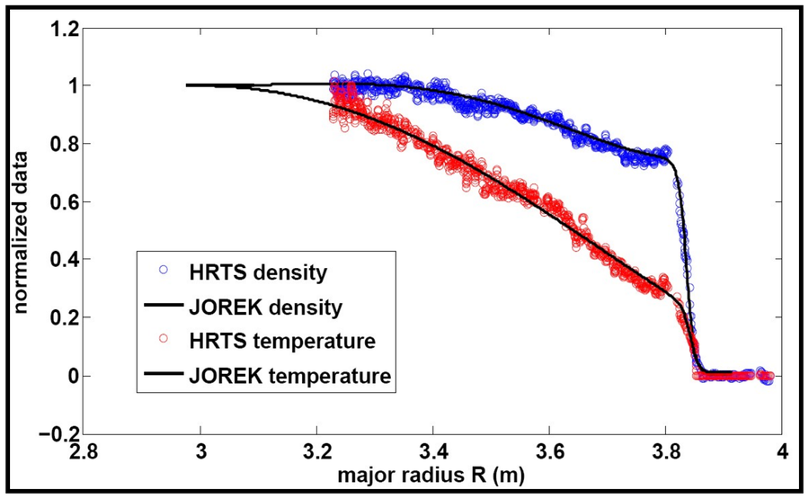
JOREK solves for density and temperature, such that the input pressure profile must be decomposed into density and temperature profiles. We will not describe here how to convert experimental data into JOREK profiles, but we will here describe the basic modified tanh profiles commonly used in JOREK. A simple way to have input profiles is just to use the num_profiles option, where you can simply feed an array profile to JOREK. For example, for the FF' profile with ffprime_file = 'jorek_ffprime.dat'.
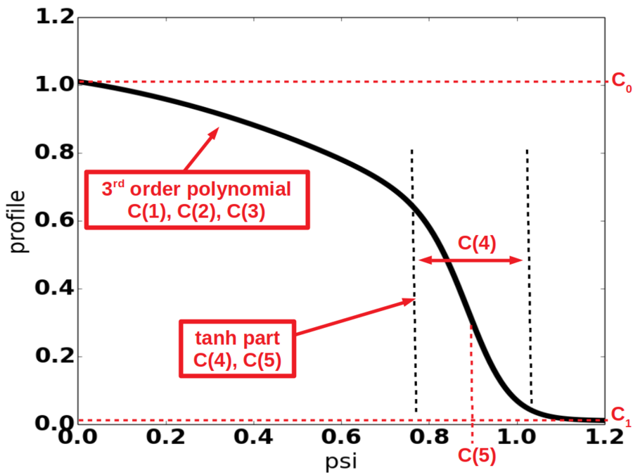
JOREK density and temperature profiles are described as modified tanh profiles:
$\rho(\psi) = (C_0-C_1) f_{poly} f_{tanh} + C_1, $ where
$f_{poly}(\psi) = 1 + C(1)\psi + C(2)\psi^2 + C(3)\psi^3$
$f_{tanh}(\psi) = 0.5 - 0.5 \tanh\left(\displaystyle\frac{\psi-C(5)}{C(4)}\right)$
The generic inputs for a JOREK profile are:
- $C_0$ : Value at magnetic axis
- $C_1$ : Value outside separatrix
- $C(1)$ : linear slope of modified tanh
- $C(2)$ : quadratic slope of modified tanh
- $C(3)$ : cubic slope of modified
- $C(4)$ : width of tanh
- $C(5)$ : position of tanh
In JOREK, the density and temperature profiles input are given as:
| density | temperature |
|---|---|
rho_0 | T_0 |
rho_1 | T_1 |
rho_coef(1) | T_coef(1) |
rho_coef(2) | T_coef(2) |
rho_coef(3) | T_coef(3) |
rho_coef(4) | T_coef(4) |
rho_coef(5) | T_coef(5) |
The FF' profile
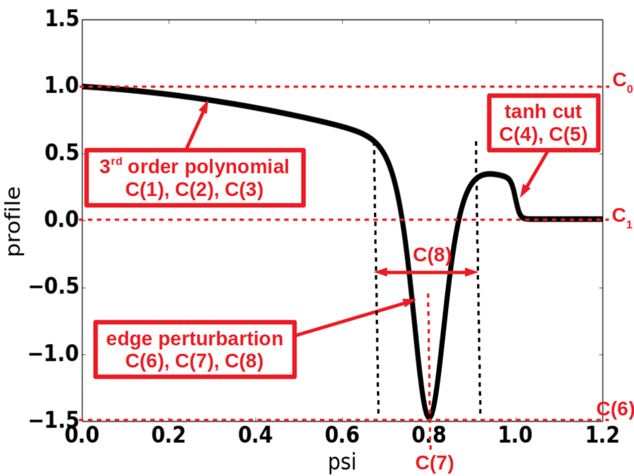
The JOREK $FF' $ profile is also a modified tanh profile, but with an additional perturbation at the plasma edge to account for the bootstrap current:
\[FF'(\psi) = \left( (C_0-C_1) f_{poly} + f_{pert}\right) f_{tanh} + C_1,\]where
\(f_{poly}(\psi) = 1 + C(1)\psi + C(2)\psi^2 + C(3)\psi^3,\) \(f_{tanh}(\psi) = 0.5 - 0.5 \tanh\left(\frac{\psi-C(5)}{C(4)}\right),\) \(f_{pert}(\psi) = \frac{C(6)}{2C(8)} \left[ \cosh\left(\frac{\psi-C(7)}{C(8)}\right)\right]^{-2}.\)
Hence, the inputs for a JOREK FF' profile are:
- $C_0$ : Value at magnetic axis
- $C_1$ : Value outside separatrix
- $C(1)$ : linear slope of modified tanh
- $C(2)$ : quadratic slope of modified tanh
- $C(3)$ : cubic slope of modified
- $C(4)$ : width of tanh (to switch off profile in SOL)
- $C(5)$ : position of tanh
- $C(6)$ : amplitude of edge perturbation
- $C(7)$ : position of edge perturbation
- $C(8)$ : width of edge perturbation
In JOREK, the FF' profile input is given as:
| FF' profile |
|---|
FF_0 |
FF_1 |
FF_coef(1) |
FF_coef(2) |
FF_coef(3) |
FF_coef(4) |
FF_coef(5) |
FF_coef(6) |
FF_coef(7) |
FF_coef(8) |
Other inputs
Note, another input required for the GS solver is F0 ($= R_0 B_{\phi}$). Note the sign convention is that a positive F0 corresponds to a toroidal magnetic field which is clockwise as seen from above. This is opposite to the standard coordinate system in ASDEX Upgrade and DIII-D, for example. Similarly, a positive current
The Polar grid
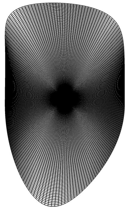
At last, the GS must be solved on an initial grid, typically a polar grid. The contour of this polar grid is given by the $\psi$-contour provided as in the first section. The centre of the grid is defined by the inputs R_geo and Z_geo. The polar grid resolution is given by n_radial and n_pol. To summarise:
| Polar grid inputs | definition |
|---|---|
R_geo | R-coord of grid centre |
Z_geo | z-coord of grid centre |
n_radial | radial resolution of the grid |
n_POL | poloidal resolution of the grid |
n_boundary | number of boundary points for edge of grid |
R_boundary(1:n_boundary) | R-coords of grid contour points |
Z_boundary(1:n_boundary) | Z-coords of grid contour points |
psi_boundary(1:n_boundary) | $\psi$-values of grid contour points |